Tidyverse 2: Data Manipulation

workflowr

• Summary
• Checks
• Past versions

Last updated: 2025-03-24

Checks: 7 0

Knit directory: analysis-user-group/

This reproducible R Markdown analysis was created with workflowr (version 1.7.1). The Checks tab describes the reproducibility checks that were applied when the results were created. The Past versions tab lists the development history.

---

R Markdown file: up-to-date

Great! Since the R Markdown file has been committed to the Git repository, you know the exact version of the code that produced these results.

Environment: empty

Great job! The global environment was empty. Objects defined in the global environment can affect the analysis in your R Markdown file in unknown ways. For reproduciblity it’s best to always run the code in an empty environment.

Seed: set.seed(1337)

The command set.seed(1337) was run prior to running the code in the R Markdown file. Setting a seed ensures that any results that rely on randomness, e.g. subsampling or permutations, are reproducible.

Session information: recorded

Great job! Recording the operating system, R version, and package versions is critical for reproducibility.

Cache: none

Nice! There were no cached chunks for this analysis, so you can be confident that you successfully produced the results during this run.

File paths: relative

Great job! Using relative paths to the files within your workflowr project makes it easier to run your code on other machines.

Repository version: 96c7594

Great! You are using Git for version control. Tracking code development and connecting the code version to the results is critical for reproducibility.

The results in this page were generated with repository version 96c7594. See the Past versions tab to see a history of the changes made to the R Markdown and HTML files.

Note that you need to be careful to ensure that all relevant files for the analysis have been committed to Git prior to generating the results (you can use wflow_publish or wflow_git_commit). workflowr only checks the R Markdown file, but you know if there are other scripts or data files that it depends on. Below is the status of the Git repository when the results were generated:

Ignored files:
    Ignored:    .DS_Store
    Ignored:    .Rhistory
    Ignored:    analysis/.DS_Store
    Ignored:    analysis/.Rhistory
    Ignored:    analysis/adit/.DS_Store

Untracked files:
    Untracked:  analysis/adit/head_index.html

Unstaged changes:
    Modified:   workflow.R

Note that any generated files, e.g. HTML, png, CSS, etc., are not included in this status report because it is ok for generated content to have uncommitted changes.

---

These are the previous versions of the repository in which changes were made to the R Markdown (analysis/202502_tidyverse2.Rmd) and HTML (docs/202502_tidyverse2.html) files. If you’ve configured a remote Git repository (see ?wflow_git_remote), click on the hyperlinks in the table below to view the files as they were in that past version.

File	Version	Author	Date	Message
html	517dcf9	DrThomasOneil	2025-03-24	Build site.
html	6a4432b	DrThomasOneil	2025-03-24	Build site.
html	1f218f3	DrThomasOneil	2025-03-24	Build site.
html	dca90e9	DrThomasOneil	2025-03-24	Build site.
html	1d1c076	DrThomasOneil	2025-03-24	Build site.
html	956ba9b	DrThomasOneil	2025-03-24	Build site.
html	d600337	DrThomasOneil	2025-03-18	Build site.
html	b537f69	DrThomasOneil	2025-03-18	Build site.
html	b7982e9	DrThomasOneil	2025-03-16	Build site.
html	fc5dd81	DrThomasOneil	2025-03-16	Build site.
html	8e1c1a3	DrThomasOneil	2025-03-16	Build site.
Rmd	d75e5ae	DrThomasOneil	2025-03-16	wflow_publish(c("analysis/*.Rmd"))
html	36dc5fc	DrThomasOneil	2025-03-03	Build site.
html	49bb28c	DrThomasOneil	2025-03-03	Build site.
html	8258922	DrThomasOneil	2025-03-03	Build site.
html	71646a5	DrThomasOneil	2025-02-27	Build site.
html	c7f5738	DrThomasOneil	2025-02-24	Build site.
html	79d09b1	DrThomasOneil	2025-02-24	Build site.
Rmd	e3febb1	DrThomasOneil	2025-02-24	wflow_publish(c("analysis/*.Rmd"))
Rmd	4a65112	DrThomasOneil	2025-02-24	Update 202502_tidyverse2.Rmd
html	a5c9f2c	DrThomasOneil	2025-02-24	Build site.
Rmd	76aec52	DrThomasOneil	2025-02-24	wflow_publish(c("analysis/*.Rmd"))
html	ca2c086	DrThomasOneil	2025-02-24	Build site.
Rmd	e2f4ac6	DrThomasOneil	2025-02-24	wflow_publish(c("analysis/*.Rmd"))
Rmd	9ab51d3	DrThomasOneil	2025-02-24	Update 202502_tidyverse2.Rmd
html	fca0503	DrThomasOneil	2025-02-24	Build site.
Rmd	c9db666	DrThomasOneil	2025-02-24	wflow_publish(c("analysis/*.Rmd"))
html	af42fba	DrThomasOneil	2025-02-24	Build site.
Rmd	24a9fef	DrThomasOneil	2025-02-24	wflow_publish(c("analysis/*.Rmd"))
html	1aeefc7	DrThomasOneil	2025-02-20	Build site.
Rmd	756ebac	DrThomasOneil	2025-02-20	wflow_publish(c("analysis/*.Rmd"))
html	5fe30de	DrThomasOneil	2025-02-20	Build site.
Rmd	477062c	DrThomasOneil	2025-02-20	wflow_publish(c("analysis/*.Rmd"))
Rmd	a48de9d	DrThomasOneil	2025-02-20	new data

---

Introduction

In this tutorial, we explore the functionalities of the Tidyverse by working with two datasets:

• data.csv contains fabricated summary flow cytometry data, such as cell numbers and MFI
• meta.csv contains information regarding each donor, such as age and sex.

The Tidyverse is a collection of R packages that share an underlying design philosophy and grammar, making data analysis more intuitive and coherent. Here are some key benefits:

dplyr: Provides a suite of verbs (e.g. filter(), mutate(), select(), and left_join()) that simplify data manipulation. For example, left_join() easily combines experimental data with metadata based on a common key. See the Introduction to R: Chapter 4 for more content on dplyr.

Pipes (%>%): Enhance code readability by allowing you to chain multiple operations in a sequential, natural-language style. This means you can finalise complex data transformations in a single, clear pipeline without the need for numerous intermediate variables.

tidyr: Focuses on tidying data, ensuring that each observation occupies a single row and each variable a single column. Functions like pivot_longer() and pivot_wider() help reshape data into a standard format, which is essential for further analysis.

ggplot2: Offers a powerful and flexible grammar for data visualisation. With ggplot2, you can create customised plots that effectively communicate insights from your data, building on the clean, tidy data produced by the other Tidyverse packages. See the Introduction to R: Chapter 5-6 and the previous workshop by Harry for extra information on ggplot.

Goals: Learn data manipulation with Tidyverse
  • Tidy Data
  • Select and Mutate data
  • Group and summarise data
  • Join two data frames
  • Pivot data with tidyr

Whether you are combining datasets, reshaping data, or creating compelling graphics, the Tidyverse offers a consistent and powerful set of tools to support your analysis.

Estimated length: 1 Hour

Set up

Follow these instructions to get started:

1. Save this script in a folder called “202502_Tidyverse2”

2. Install and load the relevant packages and functions

install.packages("tidyverse")

library(tidyverse)
theme_set(theme_classic())

2. Create new folders in your directory.

dir.create("plots")
dir.create("data")

3. Download the data.

download.file(url="https://raw.githubusercontent.com/DrThomasOneil/analysis-user-group/refs/heads/main/docs/r-tutorial/assets/synthetic_data.csv", 
              destfile = "data/data.csv", method='curl', mode='wb')
download.file(url="https://raw.githubusercontent.com/DrThomasOneil/analysis-user-group/refs/heads/main/docs/r-tutorial/assets/meta.csv", 
              destfile = "data/meta.csv", method='curl', mode='wb')

4. Load data into R

data <- read.csv("data/data.csv")
meta <- read.csv("data/meta.csv")

Data Wrangling with dplyr

First, we can quickly explore the data.

summary(data)

We have 5 categorical columns and 8 numeric values.

• CD3, CD8, CD4, HLADR and CCR5 appear to be cell counts.
  
• CD28 appears to be as a percentage already.

View(data)

Filtering, Selecting, and Mutating data: dplyr().

The dplyr package is a powerful tool for data manipulation in R. It provides a set of functions that make it easy to filter, arrange, group, and summarize data. Some of the most commonly used functions in dplyr are:

data %>% # this is the pipe. I like to think of pipes as "using this"
  head(4) %>%
  print()

  experiment  donor  tissue      layer group   CD3   CD8   CD4 HLADR  CCR5
1       Exp1 Donor1 Abdomen Epithelium   A_E  4460  2205  2184   882  1932
2       Exp1 Donor1 Abdomen Underlying  A_UM 15295  7960  5529   808  3916
3       Exp2 Donor2 Abdomen Epithelium   A_E 49774 25149 25251 10671 22763
4       Exp2 Donor2 Abdomen Underlying  A_UM 68879 47729 33616  5662 27725
  HLADR_MFI CCR5_MFI CD28
1  652.0000 4455.553 29.6
2  471.4750 7121.196 59.8
3  652.0000 3666.176 72.8
4  206.1183 2025.143 89.2

• filter(): to filter rows based on a condition

data %>%
  filter(layer == "Epithelium")%>%
  head(4) %>%
  print()

  experiment  donor  tissue      layer group    CD3   CD8   CD4 HLADR  CCR5
1       Exp1 Donor1 Abdomen Epithelium   A_E   4460  2205  2184   882  1932
2       Exp2 Donor2 Abdomen Epithelium   A_E  49774 25149 25251 10671 22763
3       Exp2 Donor3 Abdomen Epithelium   A_E 208665 92410 84610 26531 68033
4       Exp3 Donor4 Abdomen Epithelium   A_E   4460  2272  2293   985  2082
  HLADR_MFI CCR5_MFI CD28
1       652 4455.553 29.6
2       652 3666.176 72.8
3       858 7065.873 62.0
4       858 9238.000 65.6

• arrange(): to reorder rows

data %>% 
  arrange(experiment) %>%
  head(4) %>%
  print()

  experiment   donor  tissue      layer group   CD3   CD8   CD4 HLADR  CCR5
1       Exp1  Donor1 Abdomen Epithelium   A_E  4460  2205  2184   882  1932
2       Exp1  Donor1 Abdomen Underlying  A_UM 15295  7960  5529   808  3916
3       Exp1 Donor16  Vagina Epithelium   V_E 30109 17011  6596   263  6264
4       Exp1 Donor16  Vagina Underlying  V_UM 30774 16713 22180  3245 18958
  HLADR_MFI CCR5_MFI CD28
1  652.0000 4455.553 29.6
2  471.4750 7121.196 59.8
3   62.1126 3078.970 52.6
4  192.5019 3534.601  0.0

• select(): to select columns

data %>%
  filter(layer == "Epithelium") %>%
  arrange(CD4) %>%
  select(CD4) %>%
  head(4) %>%
  print()

  CD4
1 262
2 472
3 596
4 596

• mutate(): to create new columns.

data %>%
  mutate(CD4_percent = 100*CD4/CD3) %>% 
  select(CD4_percent, CD3, CD4) %>%
  head(4) %>%
  print()

  CD4_percent   CD3   CD4
1    48.96861  4460  2184
2    36.14907 15295  5529
3    50.73131 49774 25251
4    48.80443 68879 33616

Grouping and Summarising

Grouping and summarising in the Tidyverse allows you to split your data into subsets using group_by() and then compute aggregate statistics for each subgroup with summarise(). This approach enables quick, clear insights into trends and differences within your data by reducing complex datasets to meaningful summaries.

data %>%
  mutate(percent_CD4 = 100*CD4/CD3) %>%
  ggplot(aes(tissue, percent_CD4, fill=layer))+geom_boxplot()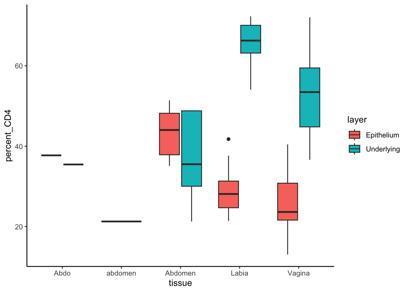

Past versions of unnamed-chunk-13-1.png

Version	Author	Date
a5c9f2c	DrThomasOneil	2025-02-24

data %>%
  mutate(percent_CD4 = 100*CD4/CD3) %>%
  group_by(tissue, layer) %>%
  summarise(mean_CD4 = mean(percent_CD4), 
            median_CD4 = median(percent_CD4)) %>%
  print()

`summarise()` has grouped output by 'tissue'. You can override using the
`.groups` argument.

# A tibble: 9 × 4
# Groups:   tissue [5]
  tissue  layer      mean_CD4 median_CD4
  <chr>   <chr>         <dbl>      <dbl>
1 Abdo    Epithelium     37.7       37.7
2 Abdo    Underlying     35.5       35.5
3 Abdomen Epithelium     43.3       44.0
4 Abdomen Underlying     37.2       35.5
5 Labia   Epithelium     28.8       28.1
6 Labia   Underlying     65.9       66.3
7 Vagina  Epithelium     26.0       23.6
8 Vagina  Underlying     52.5       53.5
9 abdomen Underlying     21.3       21.3

Joining Data Frames

Combining data from multiple sources is often necessary, even when the datasets don’t align perfectly. For instance, your long-format data might include multiple entries per donor for tissues like epithelium and mucosa, while the metadata contains donor-specific details that you prefer not to duplicate.

This scenario is common in public single cell RNA sequencing data, where you’ll integrate diverse layers of information using shared keys.

# View data values of Donor1
data[data$donor=="Donor1",]

  experiment  donor  tissue      layer group   CD3  CD8  CD4 HLADR CCR5
1       Exp1 Donor1 Abdomen Epithelium   A_E  4460 2205 2184   882 1932
2       Exp1 Donor1 Abdomen Underlying  A_UM 15295 7960 5529   808 3916
  HLADR_MFI CCR5_MFI CD28
1   652.000 4455.553 29.6
2   471.475 7121.196 59.8

# View data values of Donor1
meta[meta$donor=="Donor1",]

   donor experiment      date sex age clinical
1 Donor1       Exp1 19/2/2024   F  35  Healthy

So we expect Donor 1 to be a female, aged 35 and classified Healthy

data %>%
  select(-experiment)%>% # we can remove columns using select(-...)
  right_join(meta, by="donor") %>%
  filter(donor == "Donor1")

   donor  tissue      layer group   CD3  CD8  CD4 HLADR CCR5 HLADR_MFI CCR5_MFI
1 Donor1 Abdomen Epithelium   A_E  4460 2205 2184   882 1932   652.000 4455.553
2 Donor1 Abdomen Underlying  A_UM 15295 7960 5529   808 3916   471.475 7121.196
  CD28 experiment      date sex age clinical
1 29.6       Exp1 19/2/2024   F  35  Healthy
2 59.8       Exp1 19/2/2024   F  35  Healthy

With this, we wouldn’t need to save a combined dataframe to analyse.

data %>%
  select(-experiment)%>%
  right_join(meta, by="donor") %>%
  filter(tissue != "Abdo" & tissue != 'abdomen') %>% # remove errors
  mutate(percent = 100*CD4/CD3) %>%
  ggplot(aes(clinical, percent, fill=tissue))+
  geom_boxplot(outliers=F)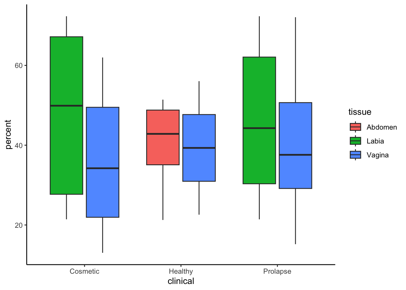

Past versions of unnamed-chunk-17-1.png

Version	Author	Date
a5c9f2c	DrThomasOneil	2025-02-24

Reshaping Data with tidyr

tidyr provides essential tools like pivot_longer() and pivot_wider() to transform your dataset between long and wide formats. This reshaping makes it easier to align variables and observations for analysis, ensuring that each variable forms a column and each observation a row. Such flexibility is crucial when preparing complex experimental or single cell RNA sequencing data for further analysis and visualisation.

long format
In long format, each observation is represented by a single row, with one column holding the categorical variable (e.g. the type of measurement) and another column holding the corresponding values. This format is particularly useful for generating boxplots or other visualisations that compare distributions across groups.

For example, if you want to compare the percentages of CD4 and CD8 cells on the same plot, you can pivot the data longer:

data %>% 
  filter(tissue != "Abdo" & tissue != 'abdomen') %>% # remove errors
  mutate(CD4percent = 100*CD4/CD3, 
         CD8percent = 100*CD8/CD3) %>%
  # pivot longer - select the columns, and the name of the columns for the names and values
  pivot_longer(cols = c(CD4percent, CD8percent), 
               names_to = "subset", 
               values_to = "percent") %>%
  select(-c(experiment,group,CCR5_MFI,HLADR_MFI,CD3,CD8,CD4,HLADR,CCR5,CD28))%>%
  head(8) %>%
  print()

# A tibble: 8 × 5
  donor  tissue  layer      subset     percent
  <chr>  <chr>   <chr>      <chr>        <dbl>
1 Donor1 Abdomen Epithelium CD4percent    49.0
2 Donor1 Abdomen Epithelium CD8percent    49.4
3 Donor1 Abdomen Underlying CD4percent    36.1
4 Donor1 Abdomen Underlying CD8percent    52.0
5 Donor2 Abdomen Epithelium CD4percent    50.7
6 Donor2 Abdomen Epithelium CD8percent    50.5
7 Donor2 Abdomen Underlying CD4percent    48.8
8 Donor2 Abdomen Underlying CD8percent    69.3

This code creates a new column subset that indicates whether the value corresponds to %CD4 or %CD8, and a column percent for the computed values. The data is now structured with one column for the measurement type and another for the percentage, making it straightforward to plot:

data %>% 
  filter(tissue != "Abdo" & tissue != 'abdomen') %>% # remove errors
  mutate(CD4percent = 100*CD4/CD3, 
         CD8percent = 100*CD8/CD3) %>%
  # pivot longer - select the columns, and the name of the columns for the names and values
  pivot_longer(cols = c(CD4percent, CD8percent), 
               names_to = "subset", 
               values_to = "percent") %>%
  ggplot(aes(layer,percent, fill=subset))+
  geom_boxplot()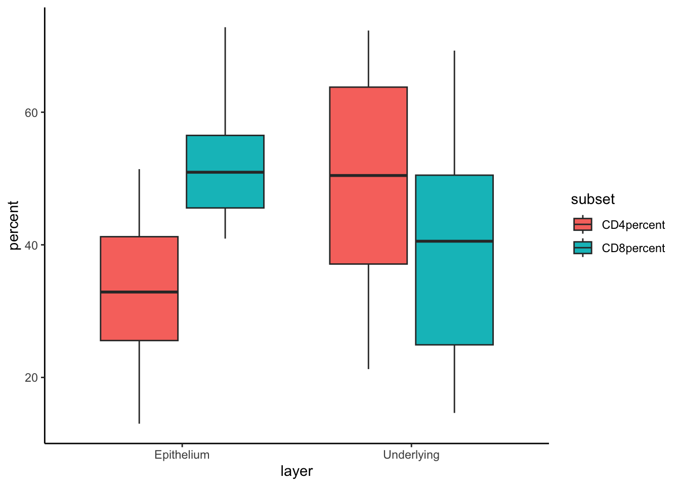

Past versions of unnamed-chunk-19-1.png

Version	Author	Date
a5c9f2c	DrThomasOneil	2025-02-24

wide format
Sometimes you want to examine relationships between measurements directly—for example, to see if there’s a relationship between values from different layers (e.g. Epithelium and Underlying mucosa). In wide format, each type of measurement occupies its own column. This structure is ideal for scatterplots or correlation analyses.

Consider this example where we pivot the data to have separate columns for each layer:

data %>% 
  filter(tissue != "Abdo" & tissue != 'abdomen') %>% # remove errors
  mutate(percent = 100*HLADR/CD4) %>%
  select(donor,tissue,layer,percent) %>%
  pivot_wider(names_from = layer, values_from = percent) %>%
  ggplot(aes(x=Epithelium, y=Underlying, color=tissue))+
    geom_point()+ 
    stat_ellipse()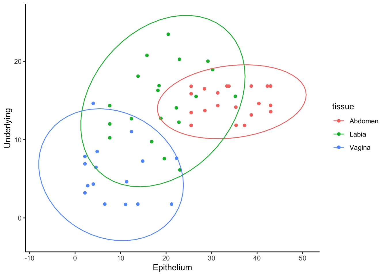

Past versions of unnamed-chunk-20-1.png

Version	Author	Date
a5c9f2c	DrThomasOneil	2025-02-24
5fe30de	DrThomasOneil	2025-02-20

Here, the pivot_wider() function converts the long data into a wide format where separate columns for Epithelium and Underlying values are created. This allows you to directly plot and explore relationships between these layers using scatterplots, with stat_ellipse() adding confidence ellipses to highlight group trends.

Both long and wide formats serve specific purposes in data analysis and visualisation. Long format is flexible for creating grouped comparisons, while wide format facilitates direct relationship analysis between variables.

Conclusions

In conclusion, this tutorial has demonstrated how the Tidyverse streamlines data analysis by providing a coherent set of tools that simplify data manipulation, reshaping, and visualisation. Using dplyr, we efficiently filtered, mutated, grouped, summarised, and joined our experimental and metadata, while the use of pipes (%>%) allowed us to finalise complex workflows in a readable and intuitive manner.

Additionally, tidyr enabled us to transform our data between long and wide formats, ensuring that it is in the optimal structure for analysis. With ggplot2, these tidy datasets were then translated into compelling graphics that highlight key patterns and relationships. Together, these tools empower analysts to create reproducible and insightful workflows, ultimately enhancing the rigour and clarity of data-driven research.

Session information

sessionInfo()

R version 4.4.0 (2024-04-24)
Platform: aarch64-apple-darwin20
Running under: macOS Sonoma 14.3

Matrix products: default
BLAS:   /Library/Frameworks/R.framework/Versions/4.4-arm64/Resources/lib/libRblas.0.dylib 
LAPACK: /Library/Frameworks/R.framework/Versions/4.4-arm64/Resources/lib/libRlapack.dylib;  LAPACK version 3.12.0

locale:
[1] en_US.UTF-8/en_US.UTF-8/en_US.UTF-8/C/en_US.UTF-8/en_US.UTF-8

time zone: Australia/Sydney
tzcode source: internal

attached base packages:
[1] stats     graphics  grDevices utils     datasets  methods   base     

other attached packages:
 [1] lubridate_1.9.4 forcats_1.0.0   stringr_1.5.1   dplyr_1.1.4    
 [5] purrr_1.0.4     readr_2.1.5     tidyr_1.3.1     tibble_3.2.1   
 [9] ggplot2_3.5.1   tidyverse_2.0.0 workflowr_1.7.1

loaded via a namespace (and not attached):
 [1] utf8_1.2.4        sass_0.4.9        generics_0.1.3    stringi_1.8.4    
 [5] hms_1.1.3         digest_0.6.37     magrittr_2.0.3    timechange_0.3.0 
 [9] evaluate_1.0.3    grid_4.4.0        fastmap_1.2.0     rprojroot_2.0.4  
[13] jsonlite_1.9.1    processx_3.8.6    whisker_0.4.1     ps_1.9.0         
[17] promises_1.3.2    httr_1.4.7        scales_1.3.0      jquerylib_0.1.4  
[21] cli_3.6.4         rlang_1.1.5       munsell_0.5.1     withr_3.0.2      
[25] cachem_1.1.0      yaml_2.3.10       tools_4.4.0       tzdb_0.5.0       
[29] colorspace_2.1-1  httpuv_1.6.15     vctrs_0.6.5       R6_2.6.1         
[33] lifecycle_1.0.4   git2r_0.35.0      fs_1.6.5          MASS_7.3-65      
[37] pkgconfig_2.0.3   callr_3.7.6       pillar_1.10.1     bslib_0.9.0      
[41] later_1.4.1       gtable_0.3.6      glue_1.8.0        Rcpp_1.0.14      
[45] xfun_0.51         tidyselect_1.2.1  rstudioapi_0.17.1 knitr_1.50       
[49] farver_2.1.2      htmltools_0.5.8.1 labeling_0.4.3    rmarkdown_2.29   
[53] compiler_4.4.0    getPass_0.2-4    

Digital Research Skills Network
Contact us